

Pangenome-based Variant Extraction
A) Necessity of Pangenome-based Variant Extraction
Conventional variant detection studies have been conducted by mapping short-read data to a single linear reference genome sequence. However, short reads are typically only 101–105 bp in length, which limits their ability to accurately detect large structural variants exceeding 500 bp. In addition, the currently widely used human reference genomes, GRCh38 and T2T-CHM13, were constructed based on specific individuals, predominantly of European ancestry, and therefore do not sufficiently reflect the unique genomic characteristics of diverse populations such as those from Africa and Southeast Asia. As a result, reads corresponding to population-specific sequences that are absent from the reference genome are not properly mapped, and variant analysis in those regions is consequently limited.
Recent advances in long-read sequencing technologies have accelerated the construction of high-quality genome assemblies, leading to the emergence of a new type of graph-based reference genome known as the pangenome. A pangenome is constructed by integrating high-quality assemblies obtained from diverse populations into a graph structure, where nodes and edges represent various types of variant information. Therefore, it can comprehensively reflect the genetic diversity of multiple populations. By utilizing such a graph-based reference genome, read mapping rates can be improved, and precise variant detection becomes possible even in population-specific genomic regions that are difficult to analyze using conventional linear reference-based approaches. Furthermore, once a pangenome is constructed, accurate genotyping of large structural variants can be achieved simply by mapping short-read data. Therefore, in this chapter, we aim to describe the overall analytical process of constructing a pangenome using high-quality genome assemblies, mapping independent short-read sequencing data to the pangenome, and extracting both small variants and structural variants.
B) Pangenome-based Variant Detection Method
-
Quality Assessment of High-quality Haploid Assemblies (Assembly QC)
Assembly-stats and QUAST are among the most commonly used programs for evaluating basic statistical metrics and overall assembly quality. Both programs generate key assembly statistics, including total length, N50 contiguity, largest contig length, and average contig length. In particular, QUAST provides the results in user-friendly formats such as PDF or HTML reports for convenient visualization and interpretation.
bash# Assembly-stats assembly-stats ${sample}.fasta > ${sample}.assembly.stats # QUAST quast.py \ ${sample}.h1.fasta ${sample}.h2.fasta \ -o ${sample}.quast.out -
Quality Assessment and Trimming of Short-read Data (Read QC)
The quality of sequencing reads greatly influences the accuracy of variant detection. In this study, FastQC was used to evaluate the overall quality of the reads, and a Phred score of 30 or higher was defined as the threshold for high-quality bases. Subsequently, Trimmomatic was used to remove adapter sequences and low-quality bases. Specifically, TruSeq3 adapter sequences were removed, bases with a Phred score below 3 were trimmed from both ends of the reads, and reads shorter than 36 bp after Phred score-based filtering were discarded.
bash# FastQC fastqc -o ${output_path} *.fastq.gz # Trimmomatic java -jar trimmomatic-0.39.jar PE \ ${sample}.R1.fastq.gz ${sample}.R2.fastq.gz \ ${sample}.paired.R1.fastq.gz ${sample}.unpaired.R1.fastq.gz \ ${sample}.paired.R2.fastq.gz ${sample}.unpaired.R2.fastq.gz \ ILLUMINACLIP:TruSeq3-PE.fa:2:30:10:2:True LEADING:3 TRAILING:3 MINLEN:36 -
Graphical Pangenome construction
The pangenome was constructed using cactus-pangenome. To run cactus-pangenome, it is mandatory to provide a working directory for the pipeline (“jobstorepath”) and an assembly information file (“sequenceFile.tsv”) that defines the set of assemblies used to build the pangenome. In sequenceFile.tsv, the first column contains the assembly name and the second column contains the absolute path to the corresponding sequence file (Table 3). For diploid assemblies, “.1” and “.2” are appended to the assembly name to clearly distinguish the two haplotypes as a pair in the table.
bashGRCh38 GRCh38.fasta sample1.1 sample1.h1.fasta sample1.2 sample1.h2.fasta sample2.1 sample2.h1.fasta sample2.2 sample2.h2.fasta sample3.1 sample3.h1.fasta sample3.2 sample3.h2.fastaCactus-pangenome first constructs a minigraph using the assemblies listed in sequenceFile.tsv and then generates a graph in Graphical Fragment Assembly (GFA) format. During this process, the “--giraffe” option enables the generation of giraffe index files (.dist and .min), which are used later for short-read mapping with vg giraffe. The indexing scope can be configured at three different levels. The “full” option builds indexes from the entire graph without any filtering. The “clip” option builds indexes from a graph in which large unaligned segments and dangling nodes have been removed. The “filter” option builds indexes from a graph where certain nodes are removed according to a haplotype frequency threshold specified by the “--filter” parameter in the script. In general, it is recommended to set the “--filter” value to approximately 10% of the total number of assemblies.
bashcactus-pangenome ./jobstorepath ./sequenceFile.tsv \ --outName ${graph} --outDir ${graph} \ --reference GRCh38 \ --filter ${N} \ --vcf --viz --odgi \ --chrom-vg clip filter --chrom-og clip filter \ --giraffe clip filter \ --gbz clip filter full \ --gfa clip full -
Align short-reads to pangenome
-
Generation of k-mer Count Data from Short-read Sequencing Data
The kmc program calculates k-mer frequency information from short-read sequencing data, and the results are output in K-mer File Format (KFF). The KFF output file is subsequently used in the short-read mapping step with vg giraffe (via the --kff-name option). Specifically, k-mer information is used to evaluate haplotypes within the graph and to remove paths that are less relevant to the sample, thereby simplifying the graph. This reduces unnecessary path exploration and improves both mapping speed and accuracy.
bashkmc -k29 -m128 -okff -t16 -hp \ -fq @sample.lst \ ${sample} \ ${TMPDIR} -
Short-read Mapping
vg giraffe performs graph-based mapping using the pangenome graph, short-read sequencing data, short-read k-mer frequency information, and graph haplotype information as inputs. Ultimately, it generates a mapping file in Graph Alignment Format (GAF), which is then compressed using bgzip.
bashvg giraffe \ -Z ${graph}.gbz \ -f ${sample}.R1.fastq.gz -f ${sample}.R2.fastq.gz \ -o gaf \ --sample ${sample} \ --progress \ --kff-name ${prefix}.kff \ --haplotype-name ${reference}.hapl \ | bgzip -c > ${sample}.${graph}.gaf.gz
-
Generation of k-mer Count Data from Short-read Sequencing Data
-
Small Variant Detection
Small variants were detected using DeepVariant, a tool specialized for small-variant calling, after projecting the GAF-format mapping information into BAM format.
-
Extracting a Specific Graph Path from the Pangenome (e.g., GRCh38)
This step extracts only a specific haplotype/path included in the full graph. In this study, only the GRCh38 path was extracted. This is an indexing step to generate (i) a list of reference paths and (ii) a linear FASTA file from the full graph.
bash# Path file generation vg paths \ --sample GRCh38 \ -L \ -x ${graph}.gbz > GRCh38.${graph}.paths.txt # Fasta file generation vg paths \ --sample GRCh38 \ --extract-fasta \ -x ${graph}.gbz > GRCh38.${graph}.fasta # Fasta index generation samtools faidx GRCh38.${graph}.fasta -
Project graph alignments
This step converts GAF-format alignments mapped to the pangenome graph into a linear reference genome of interest (e.g., GRCh38). Using vg surject, graph-coordinate–based read alignments are projected onto a specific reference path, and the results are output in BAM format. The generated BAM file can then be used for visualization in IGV and for downstream analyses with conventional linear-reference tools such as samtools and bcftools.
bashvg surject \ -x ${graph}.gbz \ -G ${sample}.${graph}.gaf.gz \ -F GRCh38.${graph}.paths.txt \ -b \ -N ${sample} \ -R "ID:${sample} LB:lib1 SM:${sample} PL:illumina PU:unit1" \ > ${sample}.GRCh38.bam -
BAM cleanup and deduplication
This step processes the surjected BAM file so that it can be treated like a standard GRCh38-aligned BAM file. It serves as a preprocessing step to facilitate downstream variant calling and consists of five stages. Specifically, based on the GRCh38 reference, the workflow includes: (1) replacing the header, (2) adding read group information, (3) sorting the BAM file, (4) removing duplicate reads, and (5) generating a BAM index file.
bash# Step 01~03 samtools reheader $DICT ${sample}.GRCh38.bam \ | samtools addreplacerg -r "@RG\tID:${sample}\tSM:${sample}\tPU:unit1" - \ | samtools sort -@ 8 -O BAM -T TMP/${sample}.tmp \ -o ${sample}.GRCh38.sort.bam.temp # Step 04 samtools rmdup \ ${sample}.GRCh38.sort.bam.temp \ ${sample}.GRCh38.sort.rmdup.bam # Step 05 samtools index -@ 2 \ ${sample}.GRCh38.sort.rmdup.bam # Remove temporary files rm -f ${sample}.GRCh38.sort.bam.temp -
DeepVariant
DeepVariant is a deep learning–based variant calling tool developed by Google. Given a BAM or CRAM file as input, it predicts SNPs and INDELs and outputs the results in VCF or gVCF format.
bashdocker run --rm --gpus all \ --workdir ${workdir} \ nvcr.io/nvidia/clara/clara-parabricks:4.4.0-1 \ pbrun deepvariant \ --ref GRCh38.${graph}.fasta \ --in-bam /workdir/${i} \ --out-variants ${sample}.GRCh38.dp.vcf.gz \ --gvcf \ --sort-by-haplotypes \ --parse-sam-aux-fields \ --mode shortread
-
Extracting a Specific Graph Path from the Pangenome (e.g., GRCh38)
-
Structure variant calling
Structural variants larger than 50 bp were detected using vg pack and vg call. Unlike the small variant detection workflow, this approach does not include a surjection step to BAM format but instead performs variant calling directly from the GAF alignment file. Although this method can also detect small variants, it is more accurate for structural variant detection.
-
Compute read support from GAM
In this step, vg pack is used to compute a compressed coverage index from the alignment results. Using the “-Q” option, the program stores, for each node, edge, and base position in the graph, the number of reads with mapping quality greater than or equal to the specified threshold (${N}).
bashvg pack \ -x ${graph}.gbz \ -Q 5 \ -a ${sample}.gaf.gz \ -o ${sample}.gaf.pack -
Graph-based SV genotyping
Variant calling is performed using vg call. In this step, homozygous reference (0/0) calls are removed to make the output VCF more compact. In addition, alleles are normalized, and the -a option is used to ensure that all snarl calls share the same coordinates and to include reference calls, thereby standardizing coordinates across samples.
bashvg call \ ${sample}.gbz \ -r ${sample}.snarls \ -k ${sample}.gaf.pack \ -s ${sample} \ -S GRCh38 \ -a \ | bgzip > ${sample}.gaf.sv.vcf.gz -
Genotype Filtering
This step filters the VCF file produced by vg call using bcftools, a program for processing and manipulating VCF files.
bash# VCF index file generation bcftools index -f ${sample}.gaf.sv.vcf.gz # Parse variants with FILTER="PASS" bcftools view \ -i 'FILTER="PASS"' \ ${sample}.gaf.sv.vcf.gz \ -Oz -o temp_${sample}.vcf.gz # Reorder the VCF header information based on the .fai file bcftools reheader \ --fai GRCh38.${graph}.fasta.fai \ -o ${sample}.gaf.sv.PASS.vcf.gz \ temp_${sample}.vcf.gz tabix -p vcf ${sample}.gaf.sv.PASS.vcf.gz # Remove variants with GT="0/0" bcftools view \ -e 'GT="0/0"' \ ${sample}.gaf.sv.PASS.vcf.gz \ -Oz -o ${sample}.gaf.sv.PASS.NoZero.vcf.gz tabix -p vcf ${sample}.gaf.sv.PASS.NoZero.vcf.gz # Remove variants with GT="0/0" or GT="./." bcftools view \ -e 'GT="0/0" | GT="./."' \ ${sample}.gaf.sv.PASS.NoZero.vcf.gz \ -Oz -o ${sample}.gaf.sv.PASS.NoZeroNoMiss.vcf.gz tabix -p vcf ${sample}.gaf.sv.PASS.NoZeroNoMiss.vcf.gz
-
Compute read support from GAM
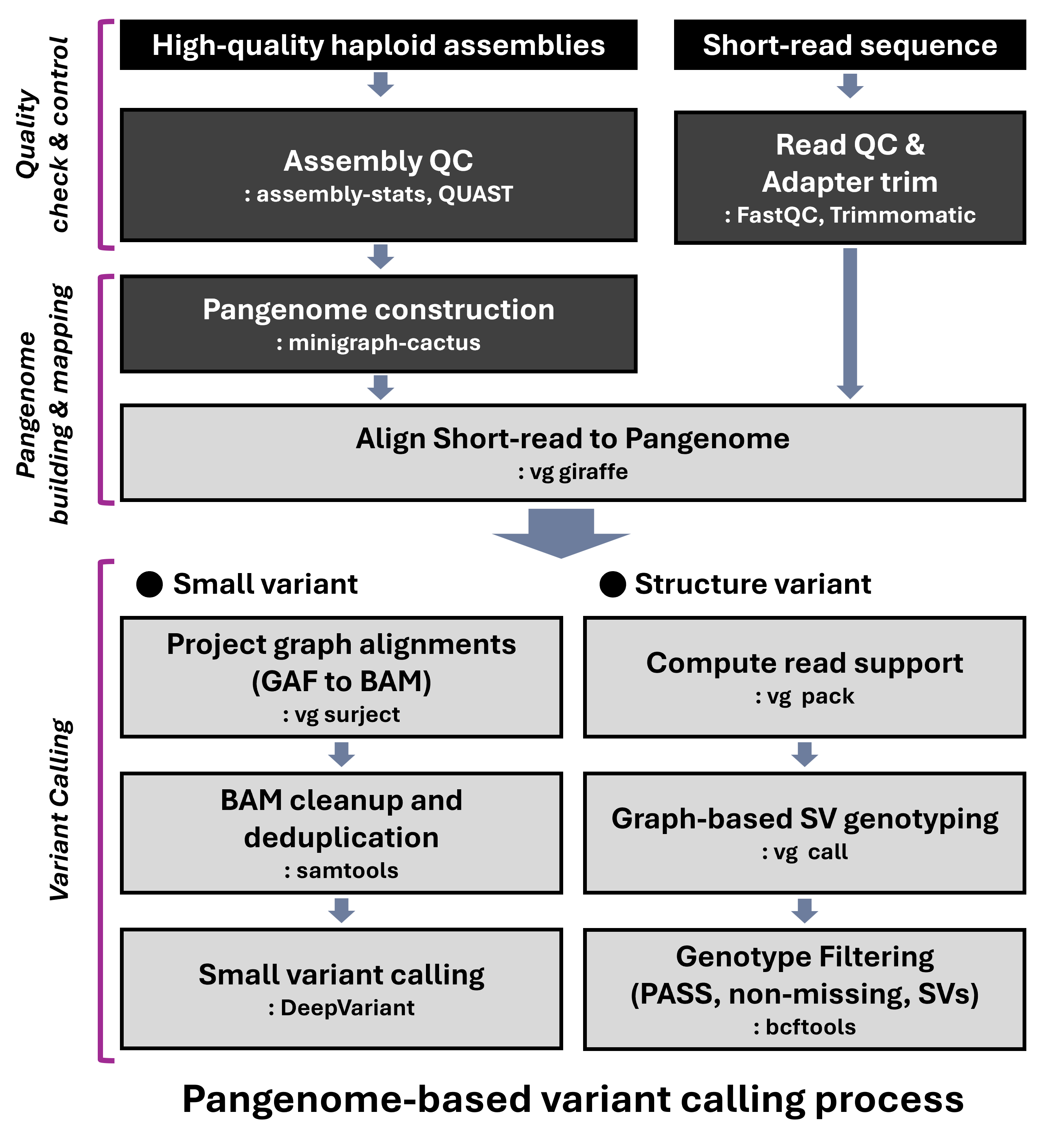
Figure 9 illustrates the overall workflow for performing pangenome-based genotyping using short-read data. The analysis proceeds in the following order: quality assessment and quality control of both genome assemblies and short-read data, construction of the pangenome, and subsequent variant detection.
C) Application of Pangenome-based Variant Information
Variant information detected through a pangenome-based approach can be applied to population genomics and evolutionary studies. In particular, population-specific structural variants identified from the pangenome graph can provide insights into how different populations have adapted to their environments. For example, if specific structural variants or copy number variations are observed at high frequencies around genes associated with high-altitude adaptation, dietary changes, or climate adaptation, this may reflect underlying adaptive mechanisms to those environments. Furthermore, by comparing allele frequency differences and haplotype structures among populations, it is possible to quantitatively analyze which genomic regions have undergone differential evolution after population divergence. In other words, pangenome-based variant data can be utilized in high-resolution evolutionary studies that integrate genetic distance, signals of selection, and gene flow among populations.
In addition, pangenome-based variant information plays an important role in the field of precision medicine. In cases of rare diseases or unexplained phenotypes, identifying causal variants within population-specific genomic sequences that are absent from conventional linear reference genomes may enable the discovery of new diagnostic markers in patients previously classified as negative. Moreover, as population-specific variant frequency data accumulate, the scope of precision medicine can expand to include assessments of population-specific disease susceptibility, prediction of drug responses, and the development of tailored therapeutic strategies. Therefore, pangenome-based variant information serves as a key resource that extends beyond fundamental evolutionary research to clinical genomics reflecting population-specific characteristics.